2017-10-09

Long-Term Charged Particle Rates from LANL GPS data

Prior posts in this series:
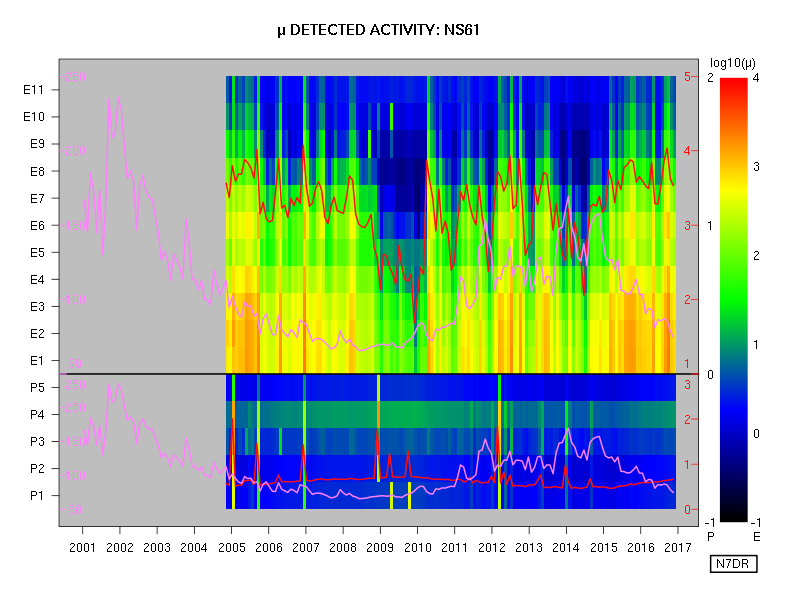
This post contains more substantial plots from the stage 35 dataset of charged particle detections from the CXD instrument aboard the GPS satellites. As in the earlier posts, the event count data are used as-is, with no attempt to impose corrections or calibrations. (Neither do I present herein any interpretations of the several interesting features that are apparent in the figures below.)

A description of the style of each plot follows the first one.


Several items of interest are plotted in a single figure. Each year is divided into twelve segments of equal duration, and data are averaged and plotted for each such bin, with time increasing in the conventional manner from left to right. The date marked on the x axis corresponds to the start of the given year.

  1. The upper panel shows data from the eleven electron channels, E1 being the lowest-energy channel and E11 the highest-energy channel. The key to the colours used is at the extreme right hand of the figure, with the logarithmic scale running from 0.1 event per second to 10,000 events per second.
  2. The lower panel shows data from the five proton channels, P1 being the lowest-energy channel and P5 the highest-energy channel. The key to the colours used is to the left of the rainbow gradient at the right of the figure, with the logarithmic scale running from 0.1 event per second to 1,000 events per second.
  3. The red wiggly line on the upper panel is the mean total event rate for electrons (i.e., over all electron channels, from E1 to E11). The scale, in events per second, is provided by the red numbers in the upper part of the grey margin that surrounds the main plotting region of the figure. The logarithmic scale runs from 10 events per second (at the black line dividing electrons from protons) to 100,000 events per second (at the top of the plotting region).
  4. The red wiggly line on the lower panel is the mean total event rate for protons (i.e., over all proton channels, from P1 to P5). The scale, in events per second, is provided by the red numbers in the lower part of the grey margin that surrounds the main plotting region of the figure. The logarithmic scale runs from 1 event per second (at the bottom of the plotting region) to 1,000 events per second (at the black line dividing electrons from protons).
  5. The purple wiggly lines on the lower and upper panels show the 10.7 cm solar flux as recorded at the Dominion Radio Astrophysical Observatory station at Penticton, British Columbia. The same data are presented in each panel: only the vertical scale differs. For each panel, the scale is given in purple at the left edge of the plotting region, and runs linearly from a flux of 50 units (which is purely notional, as the flux index never reaches such a low value), to a flux of 250 units.
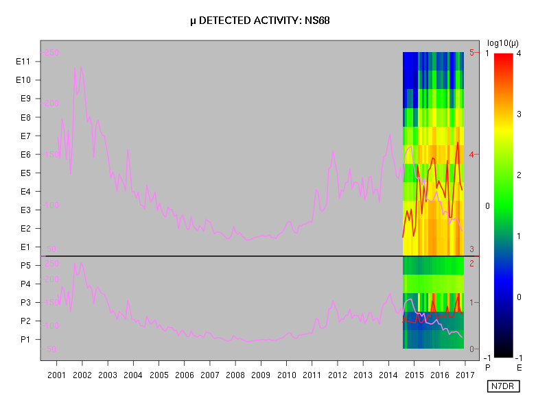
Each of the following figures is constructed similarly, one figure for each satellite carrying a CXD instrument.


2017-10-02

Improved Plots of Charged Particle Events on GPS Satellites, from LANL Public Data

This is a successor to this earlier post.

The following plots show the same information as the prior post, but with the electron and proton colour gradients scaled independently for each type of particle and each spacecraft, as well as a larger number of plottable colours, so as to provide more visible detail.

As a reminder, the plotted data are raw, taken directly from the stage 35 public dataset, with no attempt to make any corrections or calibrations.


The electron data appear much more consistent from satellite to satellite on this time scale than the proton data. Also, it is clear that some channels are more or less "sensitive" than their neighbouring channels, insofar as the raw counts reported in the dataset are concerned. Presumably, once proper calibration has been performed, the latter phenomenon will no longer be apparent.


2017-09-29

Preliminary Plots of Charged Particle Events on GPS Satellites from Public Data


Below are preliminary plots showing the electron and proton detections by the CXD instruments on the GPS satellites.

A series of posts (still unfinished) describing corrections to the originally published data is here.

Although the the corrections and amendments to the data are as yet unfinished, it is now reasonable to provide example plots of the data. The data used for the plot below are the stage 35 data, the file for which has the MD5 checksum b85d41e615126e3912bd50aa55a4af54.

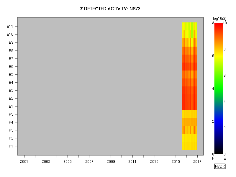
in the plots below, activity has simply been summed on a channel-by-channel basis in bins of roughly one month in duration. That is, each rectangle is coloured in accordance with the total number of recorded events in a channel over a period of roughly one month. No attempt has been made to allow for the positions of the satellites as a function of a time -- but this should be of no consequence when the summation is occurring over a period of weeks.

These plots use the data in the dataset as-is, with no attempt to modify them in any way, and all the plots use a common scale (provided next to each plot) for both electrons (the E channels) and protons (the P channels). These data are from the fields denoted rate_electron_measured and rate_proton_measured, as well as the collection_interval field. Roughly speaking, the representative energy of each channel increases with increasing channel number, although the energy ranges are quite different for the E channels and the P channels, and no attempt has been made in these plots to convert the measured numbers of events to a particle flux spectrum.

Because of the length of the binning interval, we expect the plots for all satellites to be closely similar for the time periods that they have in common.


As expected, the electron data are essentially identical for all the satellites for the periods that they have in common, and the solar cycle of activity can be seen clearly in the plots that extend for a sufficient period.

The proton data seem to show some differences from satellite to satellite, although it is possible that this is an artefact of colour gradient, which clearly is more appropriate for electrons than for protons; the plots should therefore be refined so as to provide more obvious detail in the rendering of the proton data. I leave that task for a later post.